
Note
Click here to download the full example code or to run this example in your browser via Binder
Time-related feature engineering with scikit-learn
This notebook introduces different strategies with Neuraxle to leverage time-related features for a bike sharing demand regression task that is highly dependent on business cycles (days, weeks, months) and yearly season cycles.
In the process, we introduce how to perform periodic feature engineering using
the sklearn.preprocessing.SplineTransformer class and its
extrapolation=”periodic” option.
Machine Learning Pipelines are built using the Pipeline class,
as well as ColumnTransformer
and FeatureUnion.
import matplotlib.pyplot as plt
Data exploration on the Bike Sharing Demand dataset
We start by loading the data from the OpenML repository.
import numpy as np
import pandas as pd
from neuraxle.base import Identity, MetaStep
from neuraxle.pipeline import Pipeline
from neuraxle.steps.column_transformer import ColumnTransformer
from neuraxle.union import FeatureUnion

from sklearn.datasets import fetch_openml
from sklearn.ensemble import HistGradientBoostingRegressor
from sklearn.kernel_approximation import Nystroem
from sklearn.linear_model import RidgeCV
from sklearn.model_selection import TimeSeriesSplit, cross_validate
from sklearn.preprocessing import (FunctionTransformer, MinMaxScaler,
                                   OneHotEncoder, OrdinalEncoder,
                                   PolynomialFeatures, SplineTransformer)

bike_sharing = fetch_openml("Bike_Sharing_Demand", version=2, as_frame=True)
df = bike_sharing.frame
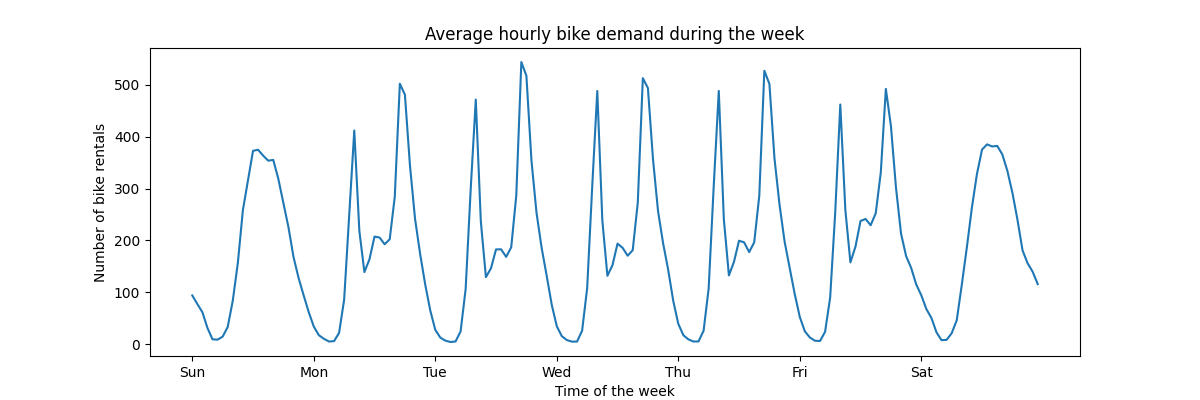
To get a quick understanding of the periodic patterns of the data, let us have a look at the average demand per hour during a week.
Note that the week starts on a Sunday, during the weekend. We can clearly distinguish the commute patterns in the morning and evenings of the work days and the leisure use of the bikes on the weekends with a more spread peak demand around the middle of the days:
fig, ax = plt.subplots(figsize=(12, 4))
average_week_demand = df.groupby(["weekday", "hour"]).mean()["count"]
average_week_demand.plot(ax=ax)
_ = ax.set(
    title="Average hourly bike demand during the week",
    xticks=[i * 24 for i in range(7)],
    xticklabels=["Sun", "Mon", "Tue", "Wed", "Thu", "Fri", "Sat"],
    xlabel="Time of the week",
    ylabel="Number of bike rentals",
)
The target of the prediction problem is the absolute count of bike rentals on a hourly basis:
df["count"].max()
Out:
977.0
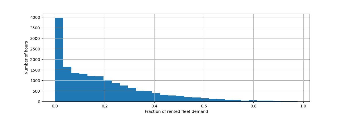
Let us rescale the target variable (number of hourly bike rentals) to predict a relative demand so that the mean absolute error is more easily interpreted as a fraction of the maximum demand.
Note
The fit method of the models used in this notebook all minimize the mean squared error to estimate the conditional mean instead of the mean absolute error that would fit an estimator of the conditional median.
When reporting performance measure on the test set in the discussion, we instead choose to focus on the mean absolute error that is more intuitive than the (root) mean squared error. Note, however, that the best models for one metric are also the best for the other in this study.
y = df["count"] / 1000
fig, ax = plt.subplots(figsize=(12, 4))
y.hist(bins=30, ax=ax)
_ = ax.set(
    xlabel="Fraction of rented fleet demand",
    ylabel="Number of hours",
)
The input feature data frame is a time annotated hourly log of variables describing the weather conditions. It includes both numerical and categorical variables. Note that the time information has already been expanded into several complementary columns.
X = df.drop("count", axis="columns")
X
Note
If the time information was only present as a date or datetime column, we could have expanded it into hour-in-the-day, day-in-the-week, day-in-the-month, month-in-the-year using pandas: https://pandas.pydata.org/pandas-docs/stable/user_guide/timeseries.html#time-date-components
We now introspect the distribution of the categorical variables, starting with “weather”:
X["weather"].value_counts()
Out:
clear         11413
misty          4544
rain           1419
heavy_rain        3
Name: weather, dtype: int64
Since there are only 3 “heavy_rain” events, we cannot use this category to train machine learning models with cross validation. Instead, we simplify the representation by collapsing those into the “rain” category.
X["weather"].replace(to_replace="heavy_rain", value="rain", inplace=True)
X["weather"].value_counts()
Out:
clear    11413
misty     4544
rain      1422
Name: weather, dtype: int64
As expected, the “season” variable is well balanced:
X["season"].value_counts()
Out:
fall      4496
summer    4409
spring    4242
winter    4232
Name: season, dtype: int64
Time-based cross-validation
Since the dataset is a time-ordered event log (hourly demand), we will use a time-sensitive cross-validation splitter to evaluate our demand forecasting model as realistically as possible. We use a gap of 2 days between the train and test side of the splits. We also limit the training set size to make the performance of the CV folds more stable.
1000 test datapoints should be enough to quantify the performance of the model. This represents a bit less than a month and a half of contiguous test data:
ts_cv = TimeSeriesSplit(
    n_splits=5,
    gap=48,
    max_train_size=10000,
    test_size=1000,
)
Let us manually inspect the various splits to check that the TimeSeriesSplit works as we expect, starting with the first split:
all_splits = list(ts_cv.split(X, y))
train_0, test_0 = all_splits[0]
X.iloc[test_0]
X.iloc[train_0]
We now inspect the last split:
train_4, test_4 = all_splits[4]
X.iloc[test_4]
X.iloc[train_4]
All is well. We are now ready to do some predictive modeling!
Gradient Boosting
Gradient Boosting Regression with decision trees is often flexible enough to efficiently handle heteorogenous tabular data with a mix of categorical and numerical features as long as the number of samples is large enough.
Here, we do minimal ordinal encoding for the categorical variables and then let the model know that it should treat those as categorical variables by using a dedicated tree splitting rule. Since we use an ordinal encoder, we pass the list of categorical values explicitly to use a logical order when encoding the categories as integers instead of the lexicographical order. This also has the added benefit of preventing any issue with unknown categories when using cross-validation.
The numerical variables need no preprocessing and, for the sake of simplicity, we only try the default hyper-parameters for this model:
categorical_columns = [
    "weather",
    "season",
    "holiday",
    "workingday",
]
non_categorical_columns = [i for i in X.columns if i not in categorical_columns]
categories = [
    ["clear", "misty", "rain"],
    ["spring", "summer", "fall", "winter"],
    ["False", "True"],
    ["False", "True"],
]
ordinal_encoder = OrdinalEncoder(categories=categories)


gbrt_pipeline = Pipeline([
    ColumnTransformer([
        (categorical_columns, ordinal_encoder),
        (non_categorical_columns, Identity()),
    ], n_dimension=2),
    HistGradientBoostingRegressor(
        categorical_features=range(4),
    ),
])
Lets evaluate our gradient boosting model with the mean absolute error of the relative demand averaged accross our 5 time-based cross-validation splits:
def evaluate(model, X, y, cv):
    class SilentMetaStep(MetaStep):
        """This class is needed here to disable the sklearn compatibility errors with the getters and setters."""

        def __init__(self):
            super().__init__(wrapped=model)

        def get_params(self, deep=False) -> dict:
            return dict()

        def set_params(self, deep=False) -> dict:
            pass
    silent_model = SilentMetaStep()
    cv_results = cross_validate(
        silent_model,
        X,
        y,
        cv=cv,
        scoring=["neg_mean_absolute_error", "neg_root_mean_squared_error"],
    )
    mae = -cv_results["test_neg_mean_absolute_error"]
    rmse = -cv_results["test_neg_root_mean_squared_error"]
    print(
        f"Evaluation results for {model}:\n\n"
        f"    Mean Absolute Error:     {mae.mean():.3f} +/- {mae.std():.3f}\n"
        f"    Root Mean Squared Error: {rmse.mean():.3f} +/- {rmse.std():.3f}\n"
    )


evaluate(gbrt_pipeline, X, y, ts_cv)
Out:
Evaluation results for Pipeline([
    ColumnTransformer([
        Pipeline([
            ColumnsSelectorND(ColumnSelector2D(name='ColumnSelector2D'), name='ColumnsSelectorND'),
            <neuraxle.steps.sklearn.SKLearnWrapper(OrdinalEncoder(...)) object 0x7f570412fca0>,
        ], name='['weather', 'season', 'holiday', 'workingday']_OrdinalEncoder'),
        Pipeline([
            ColumnsSelectorND(ColumnSelector2D(name='ColumnSelector2D'), name='ColumnsSelectorND'),
            Identity(name='Identity'),
        ], name='['year', 'month', 'hour', 'weekday', 'temp', 'feel_temp', 'humidity', 'windspeed']_Identity'),
        NumpyConcatenateInnerFeatures(name='joiner'),
    ], name='ColumnTransformer'),
    <neuraxle.steps.sklearn.SKLearnWrapper(HistGradientBoostingRegressor(...)) object 0x7f5704143580>,
], name='Pipeline'):

    Mean Absolute Error:     0.043 +/- 0.003
    Root Mean Squared Error: 0.066 +/- 0.005
This model has an average error around 4 to 5% of the maximum demand. This is quite good for a first trial without any hyper-parameter tuning! We just had to make the categorical variables explicit. Note that the time related features are passed as is, i.e. without processing them. But this is not much of a problem for tree-based models as they can learn a non-monotonic relationship between ordinal input features and the target.
This is not the case for linear regression models as we will see in the following.
Naive linear regression
As usual for linear models, categorical variables need to be one-hot encoded. For consistency, we scale the numerical features to the same 0-1 range using class:sklearn.preprocessing.MinMaxScaler, although in this case it does not impact the results much because they are already on comparable scales:
categorical_one_hot_encoders = [
    (col_name, OneHotEncoder(handle_unknown="ignore", sparse=False))
    for col_name in categorical_columns
]
alphas = np.logspace(-6, 6, 25)
naive_linear_pipeline = Pipeline([
    ColumnTransformer([
        *categorical_one_hot_encoders,
        (non_categorical_columns, MinMaxScaler()),
    ], n_dimension=2),
    RidgeCV(alphas=alphas),
])

evaluate(naive_linear_pipeline, X, y, cv=ts_cv)
Out:
Evaluation results for Pipeline([
    ColumnTransformer([
        Pipeline([
            ColumnsSelectorND(ColumnSelector2D(name='ColumnSelector2D'), name='ColumnsSelectorND'),
            <neuraxle.steps.sklearn.SKLearnWrapper(OneHotEncoder(...)) object 0x7f57041438b0>,
        ], name='weather_OneHotEncoder'),
        Pipeline([
            ColumnsSelectorND(ColumnSelector2D(name='ColumnSelector2D'), name='ColumnsSelectorND'),
            <neuraxle.steps.sklearn.SKLearnWrapper(OneHotEncoder(...)) object 0x7f5704143ca0>,
        ], name='season_OneHotEncoder'),
        Pipeline([
            ColumnsSelectorND(ColumnSelector2D(name='ColumnSelector2D'), name='ColumnsSelectorND'),
            <neuraxle.steps.sklearn.SKLearnWrapper(OneHotEncoder(...)) object 0x7f5704143f70>,
        ], name='holiday_OneHotEncoder'),
        Pipeline([
            ColumnsSelectorND(ColumnSelector2D(name='ColumnSelector2D'), name='ColumnsSelectorND'),
            <neuraxle.steps.sklearn.SKLearnWrapper(OneHotEncoder(...)) object 0x7f570413d2e0>,
        ], name='workingday_OneHotEncoder'),
        Pipeline([
            ColumnsSelectorND(ColumnSelector2D(name='ColumnSelector2D'), name='ColumnsSelectorND'),
            <neuraxle.steps.sklearn.SKLearnWrapper(MinMaxScaler(...)) object 0x7f570413d760>,
        ], name='['year', 'month', 'hour', 'weekday', 'temp', 'feel_temp', 'humidity', 'windspeed']_MinMaxScaler'),
        NumpyConcatenateInnerFeatures(name='joiner'),
    ], name='ColumnTransformer'),
    <neuraxle.steps.sklearn.SKLearnWrapper(RidgeCV(...)) object 0x7f570413d9d0>,
], name='Pipeline'):

    Mean Absolute Error:     0.139 +/- 0.014
    Root Mean Squared Error: 0.180 +/- 0.020
The performance is not good: the average error is around 14% of the maximum demand. This is more than three times higher than the average error of the gradient boosting model. We can suspect that the naive original encoding (merely min-max scaled) of the periodic time-related features might prevent the linear regression model to properly leverage the time information: linear regression does not automatically model non-monotonic relationships between the input features and the target. Non-linear terms have to be engineered in the input.
For example, the raw numerical encoding of the “hour” feature prevents the linear model from recognizing that an increase of hour in the morning from 6 to 8 should have a strong positive impact on the number of bike rentals while an increase of similar magnitude in the evening from 18 to 20 should have a strong negative impact on the predicted number of bike rentals.
Time-steps as categories
Since the time features are encoded in a discrete manner using integers (24 unique values in the “hours” feature), we could decide to treat those as categorical variables using a one-hot encoding and thereby ignore any assumption implied by the ordering of the hour values.
Using one-hot encoding for the time features gives the linear model a lot more flexibility as we introduce one additional feature per discrete time level.
hour_weekday_month = ["hour", "weekday", "month"]
non_time_non_categorical_columns = [i for i in non_categorical_columns if i not in hour_weekday_month]

time_one_hot_encoders = [
    (col_name, OneHotEncoder(handle_unknown="ignore", sparse=False))
    for col_name in hour_weekday_month
]

one_hot_linear_pipeline = Pipeline([
    ColumnTransformer([
        *categorical_one_hot_encoders,
        *time_one_hot_encoders,
        (non_time_non_categorical_columns, MinMaxScaler()),
    ], n_dimension=2),
    RidgeCV(alphas=alphas),
])

evaluate(one_hot_linear_pipeline, X, y, cv=ts_cv)
Out:
Evaluation results for Pipeline([
    ColumnTransformer([
        Pipeline([
            ColumnsSelectorND(ColumnSelector2D(name='ColumnSelector2D'), name='ColumnsSelectorND'),
            <neuraxle.steps.sklearn.SKLearnWrapper(OneHotEncoder(...)) object 0x7f5704144df0>,
        ], name='weather_OneHotEncoder'),
        Pipeline([
            ColumnsSelectorND(ColumnSelector2D(name='ColumnSelector2D'), name='ColumnsSelectorND'),
            <neuraxle.steps.sklearn.SKLearnWrapper(OneHotEncoder(...)) object 0x7f5704144070>,
        ], name='season_OneHotEncoder'),
        Pipeline([
            ColumnsSelectorND(ColumnSelector2D(name='ColumnSelector2D'), name='ColumnsSelectorND'),
            <neuraxle.steps.sklearn.SKLearnWrapper(OneHotEncoder(...)) object 0x7f5704144370>,
        ], name='holiday_OneHotEncoder'),
        Pipeline([
            ColumnsSelectorND(ColumnSelector2D(name='ColumnSelector2D'), name='ColumnsSelectorND'),
            <neuraxle.steps.sklearn.SKLearnWrapper(OneHotEncoder(...)) object 0x7f570413da30>,
        ], name='workingday_OneHotEncoder'),
        Pipeline([
            ColumnsSelectorND(ColumnSelector2D(name='ColumnSelector2D'), name='ColumnsSelectorND'),
            <neuraxle.steps.sklearn.SKLearnWrapper(OneHotEncoder(...)) object 0x7f57040dbca0>,
        ], name='hour_OneHotEncoder'),
        Pipeline([
            ColumnsSelectorND(ColumnSelector2D(name='ColumnSelector2D'), name='ColumnsSelectorND'),
            <neuraxle.steps.sklearn.SKLearnWrapper(OneHotEncoder(...)) object 0x7f57040db250>,
        ], name='weekday_OneHotEncoder'),
        Pipeline([
            ColumnsSelectorND(ColumnSelector2D(name='ColumnSelector2D'), name='ColumnsSelectorND'),
            <neuraxle.steps.sklearn.SKLearnWrapper(OneHotEncoder(...)) object 0x7f57040db280>,
        ], name='month_OneHotEncoder'),
        Pipeline([
            ColumnsSelectorND(ColumnSelector2D(name='ColumnSelector2D'), name='ColumnsSelectorND'),
            <neuraxle.steps.sklearn.SKLearnWrapper(MinMaxScaler(...)) object 0x7f57040db730>,
        ], name='['year', 'temp', 'feel_temp', 'humidity', 'windspeed']_MinMaxScaler'),
        NumpyConcatenateInnerFeatures(name='joiner'),
    ], name='ColumnTransformer'),
    <neuraxle.steps.sklearn.SKLearnWrapper(RidgeCV(...)) object 0x7f57040dbb80>,
], name='Pipeline'):

    Mean Absolute Error:     0.096 +/- 0.010
    Root Mean Squared Error: 0.128 +/- 0.010
The average error rate of this model is 10% which is much better than using the original (ordinal) encoding of the time feature, confirming our intuition that the linear regression model benefits from the added flexibility to not treat time progression in a monotonic manner.
However, this introduces a very large number of new features. If the time of
the day was represented in minutes since the start of the day instead of
hours, one-hot encoding would have introduced 1440 features instead of 24.
This could cause some significant overfitting. To avoid this we could use
sklearn.preprocessing.KBinsDiscretizer() instead to re-bin the number
of levels of fine-grained ordinal or numerical variables while still
benefitting from the non-monotonic expressivity advantages of one-hot
encoding.
Finally, we also observe that one-hot encoding completely ignores the ordering of the hour levels while this could be an interesting inductive bias to preserve to some level. In the following we try to explore smooth, non-monotonic encoding that locally preserves the relative ordering of time features.
Trigonometric features
As a first attempt, we can try to encode each of those periodic features using a sine and cosine transformation with the matching period.
Each ordinal time feature is transformed into 2 features that together encode equivalent information in a non-monotonic way, and more importantly without any jump between the first and the last value of the periodic range.
def sin_transformer(period):
    return FunctionTransformer(lambda x: np.sin(x / period * 2 * np.pi))


def cos_transformer(period):
    return FunctionTransformer(lambda x: np.cos(x / period * 2 * np.pi))
Let us visualize the effect of this feature expansion on some synthetic hour data with a bit of extrapolation beyond hour=23:
hour_df = pd.DataFrame(
    np.arange(26).reshape(-1, 1),
    columns=["hour"],
)
hour_df["hour_sin"] = sin_transformer(24).fit_transform(hour_df)["hour"]
hour_df["hour_cos"] = cos_transformer(24).fit_transform(hour_df)["hour"]
hour_df.plot(x="hour")
_ = plt.title("Trigonometric encoding for the 'hour' feature")
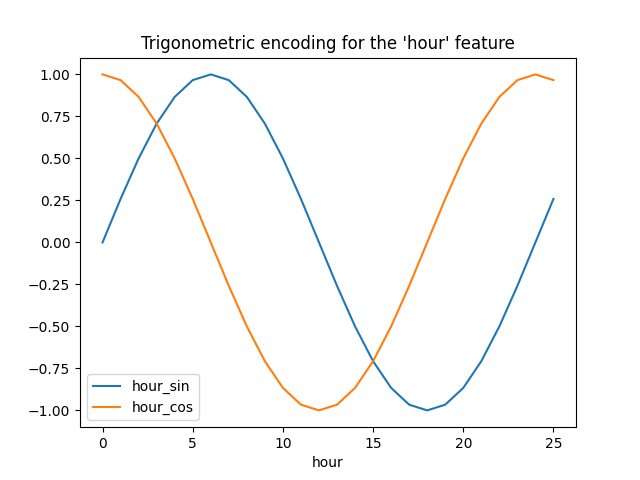
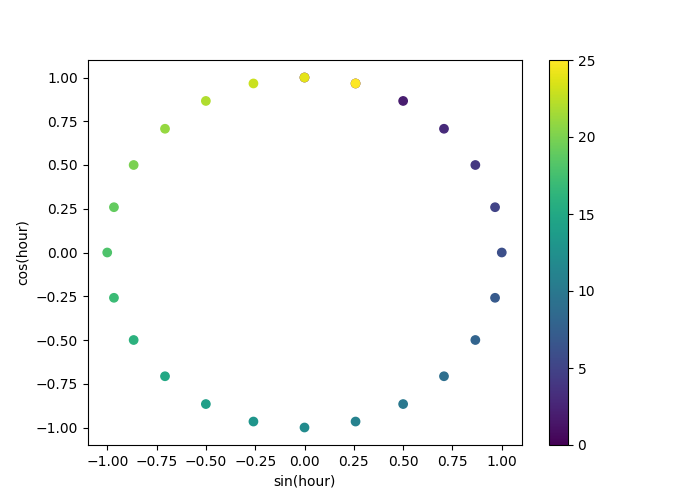
Let’s use a 2D scatter plot with the hours encoded as colors to better see how this representation maps the 24 hours of the day to a 2D space, akin to some sort of a 24 hour version of an analog clock. Note that the “25th” hour is mapped back to the 1st hour because of the periodic nature of the sine/cosine representation.
fig, ax = plt.subplots(figsize=(7, 5))
sp = ax.scatter(hour_df["hour_sin"], hour_df["hour_cos"], c=hour_df["hour"])
ax.set(
    xlabel="sin(hour)",
    ylabel="cos(hour)",
)
_ = fig.colorbar(sp)
We can now build a feature extraction pipeline using this strategy:
cyclic_cossin_transformer = ColumnTransformer([
    *categorical_one_hot_encoders,
    ("month", sin_transformer(12)),
    ("month", cos_transformer(12)),
    ("weekday", sin_transformer(7)),
    ("weekday", cos_transformer(7)),
    ("hour", sin_transformer(24)),
    ("hour", cos_transformer(24)),
    (non_time_non_categorical_columns, MinMaxScaler()),
], n_dimension=2)

cyclic_cossin_linear_pipeline = Pipeline([
    cyclic_cossin_transformer,
    RidgeCV(alphas=alphas),
])

evaluate(cyclic_cossin_linear_pipeline, X, y, cv=ts_cv)
Out:
Evaluation results for Pipeline([
    ColumnTransformer([
        Pipeline([
            ColumnsSelectorND(ColumnSelector2D(name='ColumnSelector2D'), name='ColumnsSelectorND'),
            <neuraxle.steps.sklearn.SKLearnWrapper(OneHotEncoder(...)) object 0x7f5704182f40>,
        ], name='weather_OneHotEncoder'),
        Pipeline([
            ColumnsSelectorND(ColumnSelector2D(name='ColumnSelector2D'), name='ColumnsSelectorND'),
            <neuraxle.steps.sklearn.SKLearnWrapper(OneHotEncoder(...)) object 0x7f56f879b700>,
        ], name='season_OneHotEncoder'),
        Pipeline([
            ColumnsSelectorND(ColumnSelector2D(name='ColumnSelector2D'), name='ColumnsSelectorND'),
            <neuraxle.steps.sklearn.SKLearnWrapper(OneHotEncoder(...)) object 0x7f56f87a2220>,
        ], name='holiday_OneHotEncoder'),
        Pipeline([
            ColumnsSelectorND(ColumnSelector2D(name='ColumnSelector2D'), name='ColumnsSelectorND'),
            <neuraxle.steps.sklearn.SKLearnWrapper(OneHotEncoder(...)) object 0x7f56f87a2550>,
        ], name='workingday_OneHotEncoder'),
        Pipeline([
            ColumnsSelectorND(ColumnSelector2D(name='ColumnSelector2D'), name='ColumnsSelectorND'),
            <neuraxle.steps.sklearn.SKLearnWrapper(FunctionTransformer(...)) object 0x7f56f87a28b0>,
        ], name='month_FunctionTransformer'),
        Pipeline([
            ColumnsSelectorND(ColumnSelector2D(name='ColumnSelector2D'), name='ColumnsSelectorND'),
            <neuraxle.steps.sklearn.SKLearnWrapper(FunctionTransformer(...)) object 0x7f56f87a2c10>,
        ], name='month_FunctionTransformer1'),
        Pipeline([
            ColumnsSelectorND(ColumnSelector2D(name='ColumnSelector2D'), name='ColumnsSelectorND'),
            <neuraxle.steps.sklearn.SKLearnWrapper(FunctionTransformer(...)) object 0x7f56f87a2fa0>,
        ], name='weekday_FunctionTransformer'),
        Pipeline([
            ColumnsSelectorND(ColumnSelector2D(name='ColumnSelector2D'), name='ColumnsSelectorND'),
            <neuraxle.steps.sklearn.SKLearnWrapper(FunctionTransformer(...)) object 0x7f56f87ae160>,
        ], name='weekday_FunctionTransformer1'),
        Pipeline([
            ColumnsSelectorND(ColumnSelector2D(name='ColumnSelector2D'), name='ColumnsSelectorND'),
            <neuraxle.steps.sklearn.SKLearnWrapper(FunctionTransformer(...)) object 0x7f56f87ae4c0>,
        ], name='hour_FunctionTransformer'),
        Pipeline([
            ColumnsSelectorND(ColumnSelector2D(name='ColumnSelector2D'), name='ColumnsSelectorND'),
            <neuraxle.steps.sklearn.SKLearnWrapper(FunctionTransformer(...)) object 0x7f56f87ae820>,
        ], name='hour_FunctionTransformer1'),
        Pipeline([
            ColumnsSelectorND(ColumnSelector2D(name='ColumnSelector2D'), name='ColumnsSelectorND'),
            <neuraxle.steps.sklearn.SKLearnWrapper(MinMaxScaler(...)) object 0x7f56f87aeb80>,
        ], name='['year', 'temp', 'feel_temp', 'humidity', 'windspeed']_MinMaxScaler'),
        NumpyConcatenateInnerFeatures(name='joiner'),
    ], name='ColumnTransformer'),
    <neuraxle.steps.sklearn.SKLearnWrapper(RidgeCV(...)) object 0x7f56f87aee50>,
], name='Pipeline'):

    Mean Absolute Error:     0.122 +/- 0.013
    Root Mean Squared Error: 0.162 +/- 0.019
The performance of our linear regression model with this simple feature engineering is a bit better than using the original ordinal time features but worse than using the one-hot encoded time features. We will further analyze possible reasons for this disappointing outcome at the end of this notebook.
Periodic spline features
We can try an alternative encoding of the periodic time-related features using spline transformations with a large enough number of splines, and as a result a larger number of expanded features compared to the sine/cosine transformation:
def periodic_spline_transformer(period, n_splines=None, degree=3):
    if n_splines is None:
        n_splines = period
    n_knots = n_splines + 1  # periodic and include_bias is True
    return SplineTransformer(
        degree=degree,
        n_knots=n_knots,
        knots=np.linspace(0, period, n_knots).reshape(n_knots, 1),
        extrapolation="periodic",
        include_bias=True,
    )
Again, let us visualize the effect of this feature expansion on some synthetic hour data with a bit of extrapolation beyond hour=23:
hour_df = pd.DataFrame(
    np.linspace(0, 26, 1000).reshape(-1, 1),
    columns=["hour"],
)
splines = periodic_spline_transformer(24, n_splines=12).fit_transform(hour_df)
splines_df = pd.DataFrame(
    splines,
    columns=[f"spline_{i}" for i in range(splines.shape[1])],
)
pd.concat([hour_df, splines_df], axis="columns").plot(x="hour", cmap=plt.cm.tab20b)
_ = plt.title("Periodic spline-based encoding for the 'hour' feature")
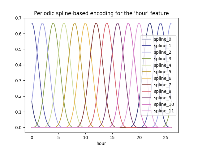
Thanks to the use of the extrapolation=”periodic” parameter, we observe that the feature encoding stays smooth when extrapolating beyond midnight.
We can now build a predictive pipeline using this alternative periodic feature engineering strategy.
It is possible to use fewer splines than discrete levels for those ordinal values. This makes spline-based encoding more efficient than one-hot encoding while preserving most of the expressivity:
cyclic_spline_transformer = ColumnTransformer([
    *categorical_one_hot_encoders,
    ("month", periodic_spline_transformer(12, n_splines=6)),
    ("weekday", periodic_spline_transformer(7, n_splines=3)),
    ("hour", periodic_spline_transformer(24, n_splines=12)),
    (non_time_non_categorical_columns, MinMaxScaler()),
], n_dimension=2)
cyclic_spline_linear_pipeline = Pipeline([
    cyclic_spline_transformer,
    RidgeCV(alphas=alphas),
])
evaluate(cyclic_spline_linear_pipeline, X, y, cv=ts_cv)
Out:
Evaluation results for Pipeline([
    ColumnTransformer([
        Pipeline([
            ColumnsSelectorND(ColumnSelector2D(name='ColumnSelector2D'), name='ColumnsSelectorND'),
            <neuraxle.steps.sklearn.SKLearnWrapper(OneHotEncoder(...)) object 0x7f56f874ee20>,
        ], name='weather_OneHotEncoder'),
        Pipeline([
            ColumnsSelectorND(ColumnSelector2D(name='ColumnSelector2D'), name='ColumnsSelectorND'),
            <neuraxle.steps.sklearn.SKLearnWrapper(OneHotEncoder(...)) object 0x7f56f874e370>,
        ], name='season_OneHotEncoder'),
        Pipeline([
            ColumnsSelectorND(ColumnSelector2D(name='ColumnSelector2D'), name='ColumnsSelectorND'),
            <neuraxle.steps.sklearn.SKLearnWrapper(OneHotEncoder(...)) object 0x7f56f86de3a0>,
        ], name='holiday_OneHotEncoder'),
        Pipeline([
            ColumnsSelectorND(ColumnSelector2D(name='ColumnSelector2D'), name='ColumnsSelectorND'),
            <neuraxle.steps.sklearn.SKLearnWrapper(OneHotEncoder(...)) object 0x7f56f8675430>,
        ], name='workingday_OneHotEncoder'),
        Pipeline([
            ColumnsSelectorND(ColumnSelector2D(name='ColumnSelector2D'), name='ColumnsSelectorND'),
            <neuraxle.steps.sklearn.SKLearnWrapper(SplineTransformer(...)) object 0x7f56f86757c0>,
        ], name='month_SplineTransformer'),
        Pipeline([
            ColumnsSelectorND(ColumnSelector2D(name='ColumnSelector2D'), name='ColumnsSelectorND'),
            <neuraxle.steps.sklearn.SKLearnWrapper(SplineTransformer(...)) object 0x7f56f8675af0>,
        ], name='weekday_SplineTransformer'),
        Pipeline([
            ColumnsSelectorND(ColumnSelector2D(name='ColumnSelector2D'), name='ColumnsSelectorND'),
            <neuraxle.steps.sklearn.SKLearnWrapper(SplineTransformer(...)) object 0x7f56f8675e80>,
        ], name='hour_SplineTransformer'),
        Pipeline([
            ColumnsSelectorND(ColumnSelector2D(name='ColumnSelector2D'), name='ColumnsSelectorND'),
            <neuraxle.steps.sklearn.SKLearnWrapper(MinMaxScaler(...)) object 0x7f56f8788340>,
        ], name='['year', 'temp', 'feel_temp', 'humidity', 'windspeed']_MinMaxScaler'),
        NumpyConcatenateInnerFeatures(name='joiner'),
    ], name='ColumnTransformer'),
    <neuraxle.steps.sklearn.SKLearnWrapper(RidgeCV(...)) object 0x7f56f867e130>,
], name='Pipeline'):

    Mean Absolute Error:     0.095 +/- 0.011
    Root Mean Squared Error: 0.129 +/- 0.012
Spline features make it possible for the linear model to successfully leverage the periodic time-related features and reduce the error from ~14% to ~10% of the maximum demand, which is similar to what we observed with the one-hot encoded features.
Qualitative analysis of the impact of features on linear model predictions
Here, we want to visualize the impact of the feature engineering choices on the time related shape of the predictions.
To do so we consider an arbitrary time-based split to compare the predictions on a range of held out data points.
naive_linear_pipeline.fit(X.iloc[train_0], y.iloc[train_0])
naive_linear_predictions = naive_linear_pipeline.predict(X.iloc[test_0])

one_hot_linear_pipeline.fit(X.iloc[train_0], y.iloc[train_0])
one_hot_linear_predictions = one_hot_linear_pipeline.predict(X.iloc[test_0])

cyclic_cossin_linear_pipeline.fit(X.iloc[train_0], y.iloc[train_0])
cyclic_cossin_linear_predictions = cyclic_cossin_linear_pipeline.predict(X.iloc[test_0])

cyclic_spline_linear_pipeline.fit(X.iloc[train_0], y.iloc[train_0])
cyclic_spline_linear_predictions = cyclic_spline_linear_pipeline.predict(X.iloc[test_0])
We visualize those predictions by zooming on the last 96 hours (4 days) of the test set to get some qualitative insights:
last_hours = slice(-96, None)
fig, ax = plt.subplots(figsize=(12, 4))
fig.suptitle("Predictions by linear models")
ax.plot(
    y.iloc[test_0].values[last_hours],
    "x-",
    alpha=0.2,
    label="Actual demand",
    color="black",
)
ax.plot(naive_linear_predictions[last_hours], "x-", label="Ordinal time features")
ax.plot(
    cyclic_cossin_linear_predictions[last_hours],
    "x-",
    label="Trigonometric time features",
)
ax.plot(
    cyclic_spline_linear_predictions[last_hours],
    "x-",
    label="Spline-based time features",
)
ax.plot(
    one_hot_linear_predictions[last_hours],
    "x-",
    label="One-hot time features",
)
_ = ax.legend()
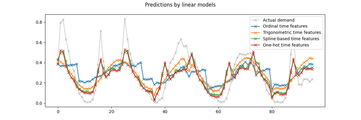
We can draw the following conclusions from the above plot:
The raw ordinal time-related features are problematic because they do not capture the natural periodicity: we observe a big jump in the predictions at the end of each day when the hour features goes from 23 back to 0. We can expect similar artifacts at the end of each week or each year.
As expected, the trigonometric features (sine and cosine) do not have these discontinuities at midnight, but the linear regression model fails to leverage those features to properly model intra-day variations. Using trigonometric features for higher harmonics or additional trigonometric features for the natural period with different phases could potentially fix this problem.
the periodic spline-based features fix those two problems at once: they give more expressivity to the linear model by making it possible to focus on specific hours thanks to the use of 12 splines. Furthermore the extrapolation=”periodic” option enforces a smooth representation between hour=23 and hour=0.
The one-hot encoded features behave similarly to the periodic spline-based features but are more spiky: for instance they can better model the morning peak during the week days since this peak lasts shorter than an hour. However, we will see in the following that what can be an advantage for linear models is not necessarily one for more expressive models.
We can also compare the number of features extracted by each feature engineering pipeline:
naive_linear_pipeline[:-1].transform(X).shape
Out:
(17379, 19)
one_hot_linear_pipeline[:-1].transform(X).shape
Out:
(17379, 59)
cyclic_cossin_linear_pipeline[:-1].transform(X).shape
Out:
(17379, 22)
cyclic_spline_linear_pipeline[:-1].transform(X).shape
Out:
(17379, 37)
This confirms that the one-hot encoding and the spline encoding strategies create a lot more features for the time representation than the alternatives, which in turn gives the downstream linear model more flexibility (degrees of freedom) to avoid underfitting.
Finally, we observe that none of the linear models can approximate the true bike rentals demand, especially for the peaks that can be very sharp at rush hours during the working days but much flatter during the week-ends: the most accurate linear models based on splines or one-hot encoding tend to forecast peaks of commuting-related bike rentals even on the week-ends and under-estimate the commuting-related events during the working days.
These systematic prediction errors reveal a form of under-fitting and can be explained by the lack of interactions terms between features, e.g. “workingday” and features derived from “hours”. This issue will be addressed in the following section.
Modeling pairwise interactions with splines and polynomial features
Linear models do not automatically capture interaction effects between input features. It does not help that some features are marginally non-linear as is the case with features constructed by SplineTransformer (or one-hot encoding or binning).
However, it is possible to use the PolynomialFeatures class on coarse grained spline encoded hours to model the “workingday”/”hours” interaction explicitly without introducing too many new variables:
hour_workday_interaction = Pipeline([
    ColumnTransformer([
        ("hour", periodic_spline_transformer(24, n_splines=8)),
        ("workingday", FunctionTransformer(lambda x: x == "True")),
    ], n_dimension=2),
    PolynomialFeatures(degree=2, interaction_only=True, include_bias=False)
])
Those features are then combined with the ones already computed in the previous spline-base pipeline. We can observe a nice performance improvemnt by modeling this pairwise interaction explicitly:
cyclic_spline_interactions_pipeline = Pipeline([
    FeatureUnion([
        cyclic_spline_transformer,
        hour_workday_interaction,
    ]),
    RidgeCV(alphas=alphas),
])
evaluate(cyclic_spline_interactions_pipeline, X, y, cv=ts_cv)
Out:
Evaluation results for Pipeline([
    FeatureUnion([
        ColumnTransformer([
            Pipeline([
                ColumnsSelectorND(ColumnSelector2D(name='ColumnSelector2D'), name='ColumnsSelectorND'),
                <neuraxle.steps.sklearn.SKLearnWrapper(OneHotEncoder(...)) object 0x7f56f874ee20>,
            ], name='weather_OneHotEncoder'),
            Pipeline([
                ColumnsSelectorND(ColumnSelector2D(name='ColumnSelector2D'), name='ColumnsSelectorND'),
                <neuraxle.steps.sklearn.SKLearnWrapper(OneHotEncoder(...)) object 0x7f56f874e370>,
            ], name='season_OneHotEncoder'),
            Pipeline([
                ColumnsSelectorND(ColumnSelector2D(name='ColumnSelector2D'), name='ColumnsSelectorND'),
                <neuraxle.steps.sklearn.SKLearnWrapper(OneHotEncoder(...)) object 0x7f56f86de3a0>,
            ], name='holiday_OneHotEncoder'),
            Pipeline([
                ColumnsSelectorND(ColumnSelector2D(name='ColumnSelector2D'), name='ColumnsSelectorND'),
                <neuraxle.steps.sklearn.SKLearnWrapper(OneHotEncoder(...)) object 0x7f56f8675430>,
            ], name='workingday_OneHotEncoder'),
            Pipeline([
                ColumnsSelectorND(ColumnSelector2D(name='ColumnSelector2D'), name='ColumnsSelectorND'),
                <neuraxle.steps.sklearn.SKLearnWrapper(SplineTransformer(...)) object 0x7f56f86757c0>,
            ], name='month_SplineTransformer'),
            Pipeline([
                ColumnsSelectorND(ColumnSelector2D(name='ColumnSelector2D'), name='ColumnsSelectorND'),
                <neuraxle.steps.sklearn.SKLearnWrapper(SplineTransformer(...)) object 0x7f56f8675af0>,
            ], name='weekday_SplineTransformer'),
            Pipeline([
                ColumnsSelectorND(ColumnSelector2D(name='ColumnSelector2D'), name='ColumnsSelectorND'),
                <neuraxle.steps.sklearn.SKLearnWrapper(SplineTransformer(...)) object 0x7f56f8675e80>,
            ], name='hour_SplineTransformer'),
            Pipeline([
                ColumnsSelectorND(ColumnSelector2D(name='ColumnSelector2D'), name='ColumnsSelectorND'),
                <neuraxle.steps.sklearn.SKLearnWrapper(MinMaxScaler(...)) object 0x7f56f8788340>,
            ], name='['year', 'temp', 'feel_temp', 'humidity', 'windspeed']_MinMaxScaler'),
            NumpyConcatenateInnerFeatures(name='joiner'),
        ], name='ColumnTransformer'),
        Pipeline([
            ColumnTransformer([
                Pipeline([
                    ColumnsSelectorND(ColumnSelector2D(name='ColumnSelector2D'), name='ColumnsSelectorND'),
                    <neuraxle.steps.sklearn.SKLearnWrapper(SplineTransformer(...)) object 0x7f56f866ed60>,
                ], name='hour_SplineTransformer'),
                Pipeline([
                    ColumnsSelectorND(ColumnSelector2D(name='ColumnSelector2D'), name='ColumnsSelectorND'),
                    <neuraxle.steps.sklearn.SKLearnWrapper(FunctionTransformer(...)) object 0x7f56f865e340>,
                ], name='workingday_FunctionTransformer'),
                NumpyConcatenateInnerFeatures(name='joiner'),
            ], name='ColumnTransformer'),
            <neuraxle.steps.sklearn.SKLearnWrapper(PolynomialFeatures(...)) object 0x7f56f86686d0>,
        ], name='Pipeline'),
        NumpyConcatenateInnerFeatures(name='joiner'),
    ], name='FeatureUnion'),
    <neuraxle.steps.sklearn.SKLearnWrapper(RidgeCV(...)) object 0x7f56f8668c10>,
], name='Pipeline'):

    Mean Absolute Error:     0.076 +/- 0.008
    Root Mean Squared Error: 0.101 +/- 0.008
Modeling non-linear feature interactions with kernels
The previous analysis highlighted the need to model the interactions between “workingday” and “hours”. Another example of a such a non-linear interaction that we would like to model could be the impact of the rain that might not be the same during the working days and the week-ends and holidays for instance.
To model all such interactions, we could either use a polynomial expansion on all marginal features at once, after their spline-based expansion. However, this would create a quadratic number of features which can cause overfitting and computational tractability issues.
Alternatively, we can use the Nyström method to compute an approximate polynomial kernel expansion. Let us try the latter:
Out:
Evaluation results for Pipeline([
    ColumnTransformer([
        Pipeline([
            ColumnsSelectorND(ColumnSelector2D(name='ColumnSelector2D'), name='ColumnsSelectorND'),
            <neuraxle.steps.sklearn.SKLearnWrapper(OneHotEncoder(...)) object 0x7f56f874ee20>,
        ], name='weather_OneHotEncoder'),
        Pipeline([
            ColumnsSelectorND(ColumnSelector2D(name='ColumnSelector2D'), name='ColumnsSelectorND'),
            <neuraxle.steps.sklearn.SKLearnWrapper(OneHotEncoder(...)) object 0x7f56f874e370>,
        ], name='season_OneHotEncoder'),
        Pipeline([
            ColumnsSelectorND(ColumnSelector2D(name='ColumnSelector2D'), name='ColumnsSelectorND'),
            <neuraxle.steps.sklearn.SKLearnWrapper(OneHotEncoder(...)) object 0x7f56f86de3a0>,
        ], name='holiday_OneHotEncoder'),
        Pipeline([
            ColumnsSelectorND(ColumnSelector2D(name='ColumnSelector2D'), name='ColumnsSelectorND'),
            <neuraxle.steps.sklearn.SKLearnWrapper(OneHotEncoder(...)) object 0x7f56f8675430>,
        ], name='workingday_OneHotEncoder'),
        Pipeline([
            ColumnsSelectorND(ColumnSelector2D(name='ColumnSelector2D'), name='ColumnsSelectorND'),
            <neuraxle.steps.sklearn.SKLearnWrapper(SplineTransformer(...)) object 0x7f56f86757c0>,
        ], name='month_SplineTransformer'),
        Pipeline([
            ColumnsSelectorND(ColumnSelector2D(name='ColumnSelector2D'), name='ColumnsSelectorND'),
            <neuraxle.steps.sklearn.SKLearnWrapper(SplineTransformer(...)) object 0x7f56f8675af0>,
        ], name='weekday_SplineTransformer'),
        Pipeline([
            ColumnsSelectorND(ColumnSelector2D(name='ColumnSelector2D'), name='ColumnsSelectorND'),
            <neuraxle.steps.sklearn.SKLearnWrapper(SplineTransformer(...)) object 0x7f56f8675e80>,
        ], name='hour_SplineTransformer'),
        Pipeline([
            ColumnsSelectorND(ColumnSelector2D(name='ColumnSelector2D'), name='ColumnsSelectorND'),
            <neuraxle.steps.sklearn.SKLearnWrapper(MinMaxScaler(...)) object 0x7f56f8788340>,
        ], name='['year', 'temp', 'feel_temp', 'humidity', 'windspeed']_MinMaxScaler'),
        NumpyConcatenateInnerFeatures(name='joiner'),
    ], name='ColumnTransformer'),
    <neuraxle.steps.sklearn.SKLearnWrapper(Nystroem(...)) object 0x7f56f8684a30>,
    <neuraxle.steps.sklearn.SKLearnWrapper(RidgeCV(...)) object 0x7f56f8684250>,
], name='Pipeline'):

    Mean Absolute Error:     0.052 +/- 0.002
    Root Mean Squared Error: 0.074 +/- 0.003
We observe that this model can almost rival the performance of the gradient boosted trees with an average error around 6% of the maximum demand.
Note that while the final step of this pipeline is a linear regression model, the intermediate steps such as the spline feature extraction and the Nyström kernel approximation are highly non-linear. As a result the compound pipeline is much more expressive than a simple linear regression model with raw features.
For the sake of completeness, we also evaluate the combination of one-hot encoding and kernel approximation:
one_hot_poly_pipeline = Pipeline([
    ColumnTransformer([
        *categorical_one_hot_encoders,
        *time_one_hot_encoders,
        (non_time_non_categorical_columns, Identity())  # passthrough
    ], n_dimension=2),
    Nystroem(kernel="poly", degree=2, n_components=300, random_state=0),
    RidgeCV(alphas=alphas)
])
evaluate(one_hot_poly_pipeline, X, y, cv=ts_cv)
Out:
Evaluation results for Pipeline([
    ColumnTransformer([
        Pipeline([
            ColumnsSelectorND(ColumnSelector2D(name='ColumnSelector2D'), name='ColumnsSelectorND'),
            <neuraxle.steps.sklearn.SKLearnWrapper(OneHotEncoder(...)) object 0x7f56f85bef40>,
        ], name='weather_OneHotEncoder'),
        Pipeline([
            ColumnsSelectorND(ColumnSelector2D(name='ColumnSelector2D'), name='ColumnsSelectorND'),
            <neuraxle.steps.sklearn.SKLearnWrapper(OneHotEncoder(...)) object 0x7f56f867eeb0>,
        ], name='season_OneHotEncoder'),
        Pipeline([
            ColumnsSelectorND(ColumnSelector2D(name='ColumnSelector2D'), name='ColumnsSelectorND'),
            <neuraxle.steps.sklearn.SKLearnWrapper(OneHotEncoder(...)) object 0x7f56f867eb20>,
        ], name='holiday_OneHotEncoder'),
        Pipeline([
            ColumnsSelectorND(ColumnSelector2D(name='ColumnSelector2D'), name='ColumnsSelectorND'),
            <neuraxle.steps.sklearn.SKLearnWrapper(OneHotEncoder(...)) object 0x7f56f867e730>,
        ], name='workingday_OneHotEncoder'),
        Pipeline([
            ColumnsSelectorND(ColumnSelector2D(name='ColumnSelector2D'), name='ColumnsSelectorND'),
            <neuraxle.steps.sklearn.SKLearnWrapper(OneHotEncoder(...)) object 0x7f56f85d35e0>,
        ], name='hour_OneHotEncoder'),
        Pipeline([
            ColumnsSelectorND(ColumnSelector2D(name='ColumnSelector2D'), name='ColumnsSelectorND'),
            <neuraxle.steps.sklearn.SKLearnWrapper(OneHotEncoder(...)) object 0x7f56f85d3100>,
        ], name='weekday_OneHotEncoder'),
        Pipeline([
            ColumnsSelectorND(ColumnSelector2D(name='ColumnSelector2D'), name='ColumnsSelectorND'),
            <neuraxle.steps.sklearn.SKLearnWrapper(OneHotEncoder(...)) object 0x7f56f85d3070>,
        ], name='month_OneHotEncoder'),
        Pipeline([
            ColumnsSelectorND(ColumnSelector2D(name='ColumnSelector2D'), name='ColumnsSelectorND'),
            Identity(name='Identity'),
        ], name='['year', 'temp', 'feel_temp', 'humidity', 'windspeed']_Identity'),
        NumpyConcatenateInnerFeatures(name='joiner'),
    ], name='ColumnTransformer'),
    <neuraxle.steps.sklearn.SKLearnWrapper(Nystroem(...)) object 0x7f56f85d3130>,
    <neuraxle.steps.sklearn.SKLearnWrapper(RidgeCV(...)) object 0x7f56f85d3190>,
], name='Pipeline'):

    Mean Absolute Error:     0.080 +/- 0.006
    Root Mean Squared Error: 0.109 +/- 0.011
While one-hot encoded features were competitive with spline-based features when using linear models, this is no longer the case when using a low-rank approximation of a non-linear kernel: this can be explained by the fact that spline features are smoother and allow the kernel approximation to find a more expressive decision function.
Let us now have a qualitative look at the predictions of the kernel models and of the gradient boosted trees that should be able to better model non-linear interactions between features:
gbrt_pipeline.fit(X.iloc[train_0], y.iloc[train_0])
gbrt_predictions = gbrt_pipeline.predict(X.iloc[test_0])

one_hot_poly_pipeline.fit(X.iloc[train_0], y.iloc[train_0])
one_hot_poly_predictions = one_hot_poly_pipeline.predict(X.iloc[test_0])

cyclic_spline_poly_pipeline.fit(X.iloc[train_0], y.iloc[train_0])
cyclic_spline_poly_predictions = cyclic_spline_poly_pipeline.predict(X.iloc[test_0])
Again we zoom on the last 4 days of the test set:
last_hours = slice(-96, None)
fig, ax = plt.subplots(figsize=(12, 4))
fig.suptitle("Predictions by non-linear regression models")
ax.plot(
    y.iloc[test_0].values[last_hours],
    "x-",
    alpha=0.2,
    label="Actual demand",
    color="black",
)
ax.plot(
    gbrt_predictions[last_hours],
    "x-",
    label="Gradient Boosted Trees",
)
ax.plot(
    one_hot_poly_predictions[last_hours],
    "x-",
    label="One-hot + polynomial kernel",
)
ax.plot(
    cyclic_spline_poly_predictions[last_hours],
    "x-",
    label="Splines + polynomial kernel",
)
_ = ax.legend()
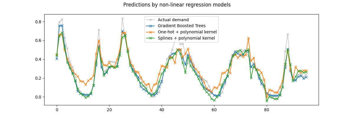
First, note that trees can naturally model non-linear feature interactions since, by default, decision trees are allowed to grow beyond a depth of 2 levels.
Here, we can observe that the combinations of spline features and non-linear kernels works quite well and can almost rival the accuracy of the gradient boosting regression trees.
On the contrary, one-hot encoded time features do not perform that well with the low rank kernel model. In particular, they significantly over-estimate the low demand hours more than the competing models.
We also observe that none of the models can successfully predict some of the peak rentals at the rush hours during the working days. It is possible that access to additional features would be required to further improve the accuracy of the predictions. For instance, it could be useful to have access to the geographical repartition of the fleet at any point in time or the fraction of bikes that are immobilized because they need servicing.
Let us finally get a more quantative look at the prediction errors of those three models using the true vs predicted demand scatter plots:
fig, axes = plt.subplots(ncols=3, figsize=(12, 4), sharey=True)
fig.suptitle("Non-linear regression models")
predictions = [
    one_hot_poly_predictions,
    cyclic_spline_poly_predictions,
    gbrt_predictions,
]
labels = [
    "One hot + polynomial kernel",
    "Splines + polynomial kernel",
    "Gradient Boosted Trees",
]
for ax, pred, label in zip(axes, predictions, labels):
    ax.scatter(y.iloc[test_0].values, pred, alpha=0.3, label=label)
    ax.plot([0, 1], [0, 1], "--", label="Perfect model")
    ax.set(
        xlim=(0, 1),
        ylim=(0, 1),
        xlabel="True demand",
        ylabel="Predicted demand",
    )
    ax.legend()
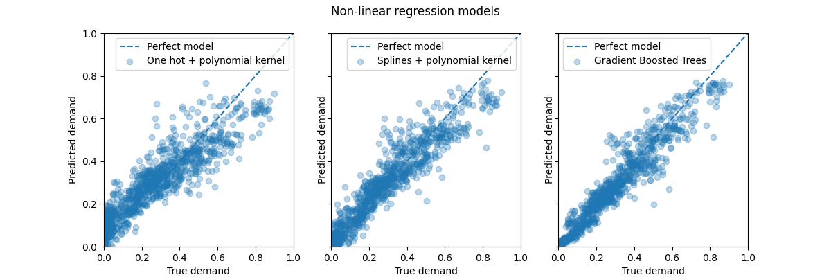
This visualization confirms the conclusions we draw on the previous plot.
All models under-estimate the high demand events (working day rush hours), but gradient boosting a bit less so. The low demand events are well predicted on average by gradient boosting while the one-hot polynomial regression pipeline seems to systematically over-estimate demand in that regime. Overall the predictions of the gradient boosted trees are closer to the diagonal than for the kernel models.
Concluding remarks
We note that we could have obtained slightly better results for kernel models by using more components (higher rank kernel approximation) at the cost of longer fit and prediction durations. For large values of n_components, the performance of the one-hot encoded features would even match the spline features.
The Nystroem + RidgeCV regressor could also have been replaced by
MLPRegressor with one or two hidden layers
and we would have obtained quite similar results.
The dataset we used in this case study is sampled on a hourly basis. However cyclic spline-based features could model time-within-day or time-within-week very efficiently with finer-grained time resolutions (for instance with measurements taken every minute instead of every hours) without introducing more features. One-hot encoding time representations would not offer this flexibility.
Finally, in this notebook we used RidgeCV because it is very efficient from a computational point of view. However, it models the target variable as a Gaussian random variable with constant variance. For positive regression problems, it is likely that using a Poisson or Gamma distribution would make more sense. This could be achieved by using GridSearchCV(TweedieRegressor(power=2), param_grid({“alpha”: alphas})) instead of RidgeCV.
Source
Note
Some of the code in the current file is adapted from the following scikit-learn documentation example, and was updated to Neuraxle code for demonstration herein. Here is the license of the original example:
BSD 3-Clause License
Copyright (c) 2007-2021 The scikit-learn developers. All rights reserved.
Redistribution and use in source and binary forms, with or without modification, are permitted provided that the following conditions are met:
Redistributions of source code must retain the above copyright notice, this
list of conditions and the following disclaimer.
Redistributions in binary form must reproduce the above copyright notice,
this list of conditions and the following disclaimer in the documentation and/or other materials provided with the distribution.
Neither the name of the copyright holder nor the names of its
contributors may be used to endorse or promote products derived from this software without specific prior written permission.
THIS SOFTWARE IS PROVIDED BY THE COPYRIGHT HOLDERS AND CONTRIBUTORS “AS IS” AND ANY EXPRESS OR IMPLIED WARRANTIES, INCLUDING, BUT NOT LIMITED TO, THE IMPLIED WARRANTIES OF MERCHANTABILITY AND FITNESS FOR A PARTICULAR PURPOSE ARE DISCLAIMED. IN NO EVENT SHALL THE COPYRIGHT HOLDER OR CONTRIBUTORS BE LIABLE FOR ANY DIRECT, INDIRECT, INCIDENTAL, SPECIAL, EXEMPLARY, OR CONSEQUENTIAL DAMAGES (INCLUDING, BUT NOT LIMITED TO, PROCUREMENT OF SUBSTITUTE GOODS OR SERVICES; LOSS OF USE, DATA, OR PROFITS; OR BUSINESS INTERRUPTION) HOWEVER CAUSED AND ON ANY THEORY OF LIABILITY, WHETHER IN CONTRACT, STRICT LIABILITY, OR TORT (INCLUDING NEGLIGENCE OR OTHERWISE) ARISING IN ANY WAY OUT OF THE USE OF THIS SOFTWARE, EVEN IF ADVISED OF THE POSSIBILITY OF SUCH DAMAGE.
Total running time of the script: ( 0 minutes 14.253 seconds)